Project Description
Introduction
The impact of Arctic sea ice decline (e.g., Perovich & Richter-Menge 2009, Meier 2017) on future global tidal and storm surge extreme water levels is unknown. Regional studies show that the impact can be substantial (e.g., Kowalik 1981, Overeem et al. 2011) causing increased erosion (e.g., Barnhart et al. 2014) and posing increased risks to fragile Arctic ecosystems in low-lying areas (e.g., Kokelj et al. 2012). Because Arctic tides and surges impact North Sea water levels, the impact will also be noticed in the Dutch coastal waters and Wadden Sea. Especially for the Wadden Sea this urges the need to quantify the impact as any change impacts the dynamics of this tidal inlet system (e.g., Chang et al. 2007, De Swart & Zimmerman 2009) and as such influences the existing ecosystem (Dittmann 1999, Blauw et al. 2012). To quantify the impact, we need to develop an accurate Arctic/global total water level (TWL) model rather than to rely on existing Arctic/global ocean tide models and storm surge models. Only for a TWL model we can complement the very limited number of tide gauge records available in the Arctic waters by the wealth of satellite radar altimeter data, which is indispensable to calibrate the model for the large uncertainties in the bathymetry and other model parameters. Indeed, when calibrating the model using TWLs there is no longer the need to decompose the altimeter TWLs into its tidal and non-tidal contributions. Strictly speaking, the latter is not possible in the Arctic based on harmonic analysis of altimeter water level time series (Parke et al. 1987). This paradigm shifting approach of using TWLs in calibrating a hydrodynamic model was proposed first by the research team and successfully applied using tide gauge data to calibrate the current operational Dutch storm surge model (Zijl et al., 2013). The first main objective (RO1) of this project is to extend the approach and apply it to calibrate a new Arctic TWL model using altimeter-derived TWLs. Thereafter, the calibrated Arctic TWL model will be used to assess the impact of Arctic sea ice decline on global tides and surges with special focus on the Arctic and the North Sea (RO2), and to improve storm surge forecasting in the Netherlands (RO3).
Current Status
No Arctic TWL model is available
Currently, no TWL model or TWL data product (via, e.g., the Copernicus Marine Environment
Monitoring Service) covering the entire Arctic Ocean is publicly available. Available are: ocean circulation models
(e.g., Madec 2008), tide models (e.g., Stammer et al. 2014), and surge models (e.g., Lynch and Gray 1979) that all
describe part of the TWL. However, as the physics described by these models overlap, no TWL data product can be obtained
by summing these three components.
Arbic et al. (2010, 2012) were the first who attempted to develop a global TWL model. However, their model was not
tailored to the Arctic. They used a high-resolution version of the ocean circulation model HYbrid Coordinate Ocean Model
(HYCOM), which Arbic et al. (2010, 2012) extend with tides.
Verlaan et al. (2015) developed the Global Tide and Surge Model (GTSM). By adding the baroclinic water levels using
the approach developed by Slobbe et al. (2013a), this model is turned into a TWL model. GTSM is being used to study
the impact of climate change on storm surges and extreme water levels (e.g., Muis et al. 2016) and to provide boundary
conditions for high-resolution regional models.
Arctic sea ice decline has an impact on tides and surges
Ongoing climate change affects tides and surges. For example, Pickering et al. (2017)
showed that globally there will be a strong response of tidal amplitudes to sea level rise. Vousdoukas et al. (2017)
showed that future extreme sea levels and flood risk along European coasts will be strongly impacted by global warming.
The main driver of the projected rise in extreme sea levels is the relative sea level rise. In their study, the North
Sea region is projected to face the highest increase in extreme sea levels. In the Arctic, it has been shown that
warming is increasing the frequency and intensity of storms (ACIA 2005, Atkinson 2005, Manson and Solomon 2007,
Sepp and Jaagus 2011, Vermaire et al. 2013).
A limited number of studies are devoted to the impact of Arctic sea ice decline on tides and surges.
Overeem et al. (2011) and Lintern et al. (2011) showed that the reduced sea ice extent provides greater fetch and
wave action and as such allows higher storm surges to reach the shore. Several authors have shown that ice cover
alters the (local) tides (e.g., Kowalik & Untersteiner 1978, Murty 1985, Godin 1986). Some specifically addressed
the impact of seasonal ice cover variations on tides (e.g., Godin 1986, St-Laurent et al. 2008, Kagan & Sofina 2010).
The latter found the largest sensitivity on the Siberian continental shelf, where seasonal changes of the M2 tidal
amplitude are estimated to be ±5 cm, while those of the M2 tidal phase vary from 15° to several tens of degrees.
We are aware of only one study from which the potential impact of the disappearance of the Arctic sea ice on tides
can be inferred. Kowalik (1981) computed the M2 co-tidal chart for the ice-free and ice-covered Arctic ocean. The
additional friction induced by the ice cover turned out to have only a minor effect on the amplitude of the tide
in the deeper part of the Arctic Ocean. In shallower waters, a more pronounced effect (decimeters) was found.
Arctic tides and surges have an impact on water levels in the North Sea
The Dutch Continental Shelf Model version 6 (DCSMv6) is the backbone of the operational
storm surge forecasting system in the Netherlands. Its northern boundary is close to the Arctic circle
(Zijl et al., 2013). Along this boundary (forecasted) Arctic tide and surge water levels serve as open boundary
conditions.
The DCSMv6 solves the depth-integrated barotropic shallow water equations assuming that the water density is uniform
in both space and time. In the North Sea, this is a justified approximation for describing the dominating tidal and
surge water levels; the water level variations induced by time-dependent baroclinic pressure gradients (e.g. due to
the Rhine Region of Freshwater Influence and salinity intrusion in rivers and estuaries) are much smaller. The model
was calibrated using TWLs acquired at a number of tide gauges from which the mean was replaced by a model-derived mean
water level to account for the missing baroclinic forcing (Zijl et al., 2013). The accuracy of the model in terms of
root-mean-square error is currently ~7-8 cm (Zijl et al. 2015).
DCSMv6 was developed to forecast storm surge water levels, but the model has many other applications. Frederikse et
al. (2016) used DCSMv6 to estimate the North Sea decadal sea level variability from tide gauge records. In the recently
finished STW project 12553 “Vertical Reference Frame for the Netherlands Mainland, Wadden Island and Continental Shelf
(NEVREF)” managed by team member Klees, the missing baroclinic forcing has been added. More specific, the model has
been extended to account for the depth-averaged horizontal water density variations and the net expansion/ contraction
of the water column (Slobbe et al. 2013a). By doing so the model provides TWLs that can be directly compared to
altimeter-observed water levels. Based on the extended model, a number of novel applications have been developed.
These include: i) chart datum realization (Slobbe et al. 2013b, 2014a), ii) quasi-geoid modeling using satellite
radar altimetry (Slobbe et al. 2014b, Farahani et al. 2016), and iii) model-based hydrodynamic leveling
(Slobbe et al. 2016).
Motivation
Calibration of an Arctic TWL model allows a direct use of altimeter-observed total water levels
The most important and problematic step in the development of an Arctic TWL model is
the calibration. Calibration is needed to limit the propagation of uncertainties in the bathymetry, model parameters
(e.g. bottom friction), and parameterizations used, and hence to obtain a more realistic state of the system as well
as more reliable and accurate reconstructions and forecasts of the Arctic water levels. Tidal and non-tidal parts are
traditionally calibrated in two separate steps (e.g., Verboom et al. 1992; Mouthaan et al. 1994; Gerritsen et al. 1995;
Philippart et al. 1998). In the first step, the model is calibrated to reconstruct the astronomical tide based on
observation-derived tidal water levels. Here, typically the model bathymetry, bottom friction coefficients, and open
boundary conditions are calibrated. In the second step, atmospheric pressure and wind forcing are added, and a
calibration of the Charnock coefficient is conducted using TWLs (indeed, the time-varying baroclinic water levels are
ignored). To calibrate an Arctic TWL model, the key problem of this method is that it requires a decomposition of the
observed water levels into its tidal and non-tidal contributions. Poleward of the TOPEX/Poseidon and Jason maximum
latitude (i.e. > 66°) direct tidal analysis of altimeter measurements is not possible, since the radar altimeter
observations that cover the higher latitudes are all sun-synchronous and thus contain serious aliasing issues when used
for tidal analysis (Parke et al. 1987). This leaves tide gauges, but they are sparsely available in the Arctic waters.
We propose to calibrate all parameters using TWLs observed by both tide gauges and satellite altimeters. We were the
first who developed such an approach, and successfully calibrated the DCSMv6 (Zijl et al. 2013), at that time using
exclusively tide gauge records, which are abundantly available in the North Sea. Here, we will specifically focus on
the use of satellite radar altimeter data. The use of these data is challenging due to their poor temporal resolution.
The impact of Arctic sea ice decline on future global tides and surges is not known yet
Past research showed that the Arctic sea ice decline has an impact on tides and
surges. We will be the first to quantify this impact on a global scale. The work of Kowalik (1981) was limited in
scope as it only considered the impact on the M2 tide (no other constituents and no surge) and for the Arctic Ocean.
Moreover, this study was conducted before the satellite altimetry era over which our knowledge of the ocean tides
has improved dramatically. Similar arguments apply to the other cited studies in which effects of sea ice cover on
tides and surges is quantified. The models used in the recent studies of Pickering et al. (2017) and Vousdoukas et
al. (2017) do not even include ice cover let alone their future projections account for the impact of the Arctic
sea ice decline. Based on the results presented in case study 1, we believe that this simplification is not
justified.
Case study 1: M2 co-tidal charts
Originally, the GTSM’s bathymetry was solely derived from the General Bathymetric
chart of the Oceans (GEBCO). In the ice-covered waters around Antarctica, however, GEBCO contains the height of
the ice surface rather than the bathymetry below the ice. Consequently, these waters were incorrectly flagged as
land ice. The resulting M2 co-tidal chart is shown in Fig. 1a. In Fig. 1b, again the M2
co-tidal chart is shown but now after updating the bathymetry using the BedMap2 data set (Fretwell et al. 2013)
that includes the ice-thickness and the bathymetry below the ice shelves. To compute Fig. 1b, we accounted for
the ice thickness, but not for ice stiffness and energy dissipation. The impact of these local changes is
remarkably large. The amplitude of the M2 constituent changes by more than a meter in the Weddell Sea.
Changes of several decimeters are observed even in the North Atlantic. Clearly, changes to tides can have an
influence over very long distances.
-
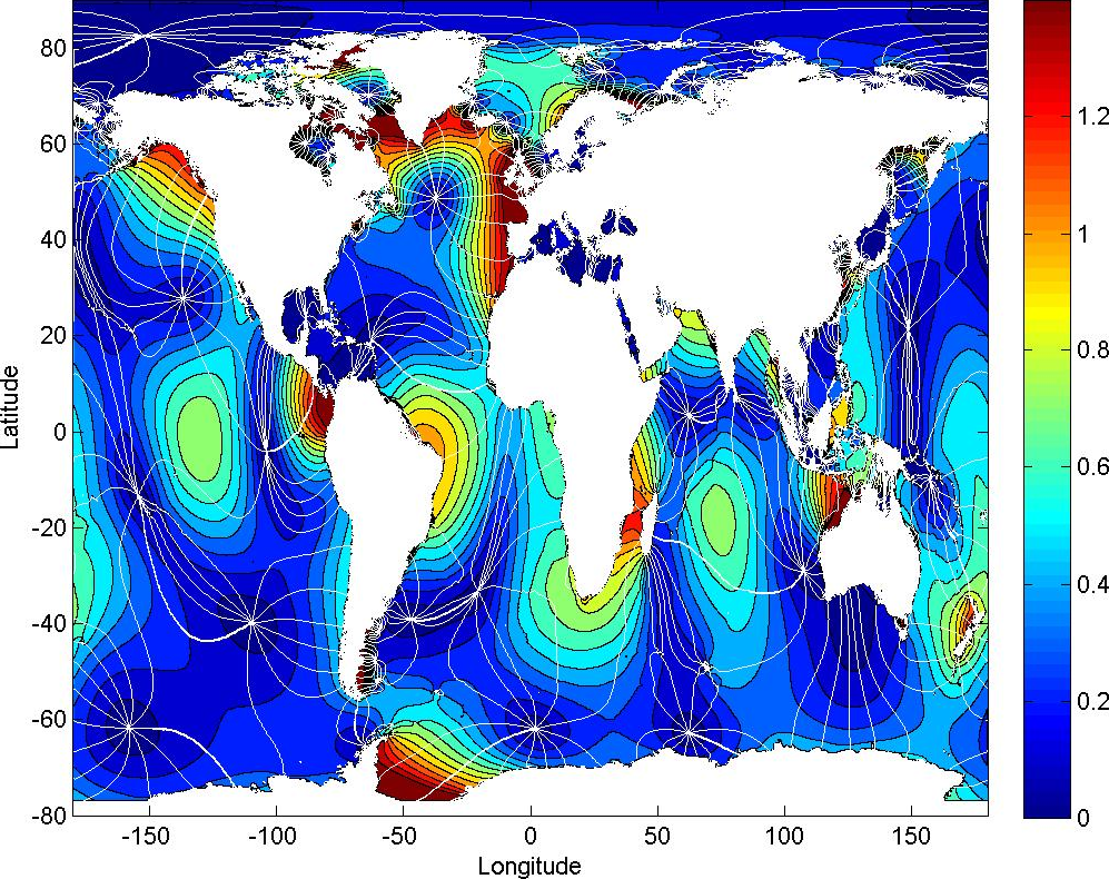
Fig. 1a: M2 co-tidal chart obtained with GEBCO bathymetry.
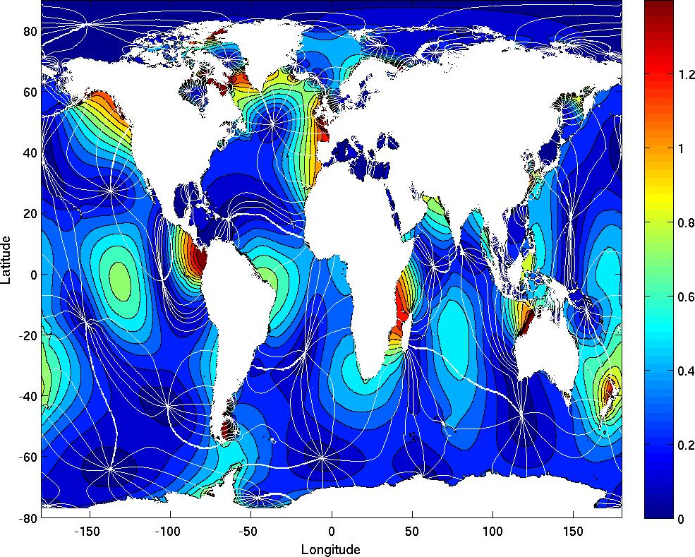
Fig. 1b: M2 co-tidal chart obtained after updating the model bathymetry around Antarctica using the BedMap2 data set.
The current approximation of Arctic surge water levels is a primary error source in operational storm surge forecasting in the Netherlands
Forecasted Arctic tidal and surge water levels serve as open boundary conditions in operational storm surge forecasting in the Netherlands. The surge water levels being more important than tides for this application. Tides are believed to be very accurate as all boundaries are still within the latitudinal range covered by the TOPEX/Poseidon and Jason-1/2 satellite radar altimeter missions. The surge water levels have always been approximated by the inverted barometer correction (IBC), in which a static oceanic response to the atmospheric load is assumed, and in which wind effects are totally ignored (Jeffreys 1916). Wunsch and Stammer (1997) showed that this is a valid assumption in most of the deep oceans except in the tropics and in the western boundary current extension regions. Mathers and Woodworth (2001) found a similar result, but they state: ”However, several parts of the Southern Ocean and other higher-latitude areas were seen from the altimetry to contain significant departures across the range of timescales accessible for study by the technique”. With a preliminary experiment, we obtained a better reconstruction of the observed water levels when including in the open boundary conditions the wind-induced water levels (see case study 2). How this has to be interpreted is still an open question. We conclude that these results confirm that Arctic surge water levels impact surge water levels in the North Sea. Furthermore, we conclude that with the current accuracy level, the approximation of the surge water level using the IBC is one of the primary error sources.
Case study 2: reconstruction of the observed water level in Den Helder during the storm on March 1, 2008
-
To assess whether wind-induced water level variations along the open sea boundaries affect the modeled water levels along the Dutch coast, we did a preliminary reconstruction of the water levels during the storm on March 1, 2008 (Stormvloedwaarschuwingsdienst, 2008) using two model setups. They differ from each other in the way the surge water levels along the open sea boundaries were formulated, i.e., either using the inverted barometer correction (IBC) or using the dynamic atmospheric correction (DAC) data set (Carrère and Lyard 2003). The DAC combines the high frequencies of the MOG2D barotropic model (Lynch and Gray 1979) forced by pressure and wind [from the European Centre for Medium-Range Weather Forecasts (ECMWF) analysis] with the low frequencies of the IBC. Figure 2 shows that the differences between the IBC and DAC increase towards the north. The RMS difference is about 5 cm. During a storm, the differences between the IBC and DAC can be much larger. In the days just before and after the storm on March 1, 2008 the peak-to-peak differences in the north are > 20 cm (see Fig. 3). In Fig. 4, we show the impact for tide gauge Den Helder. We observe that the use of the IBC to formulate the open boundary conditions results in a reconstruction error of the maximum water level of ~10 cm. When using the DAC this error is ~5 cm, i.e., a reduction of ~50%. We aim at a further reduction of these errors in the framework of this project.
-
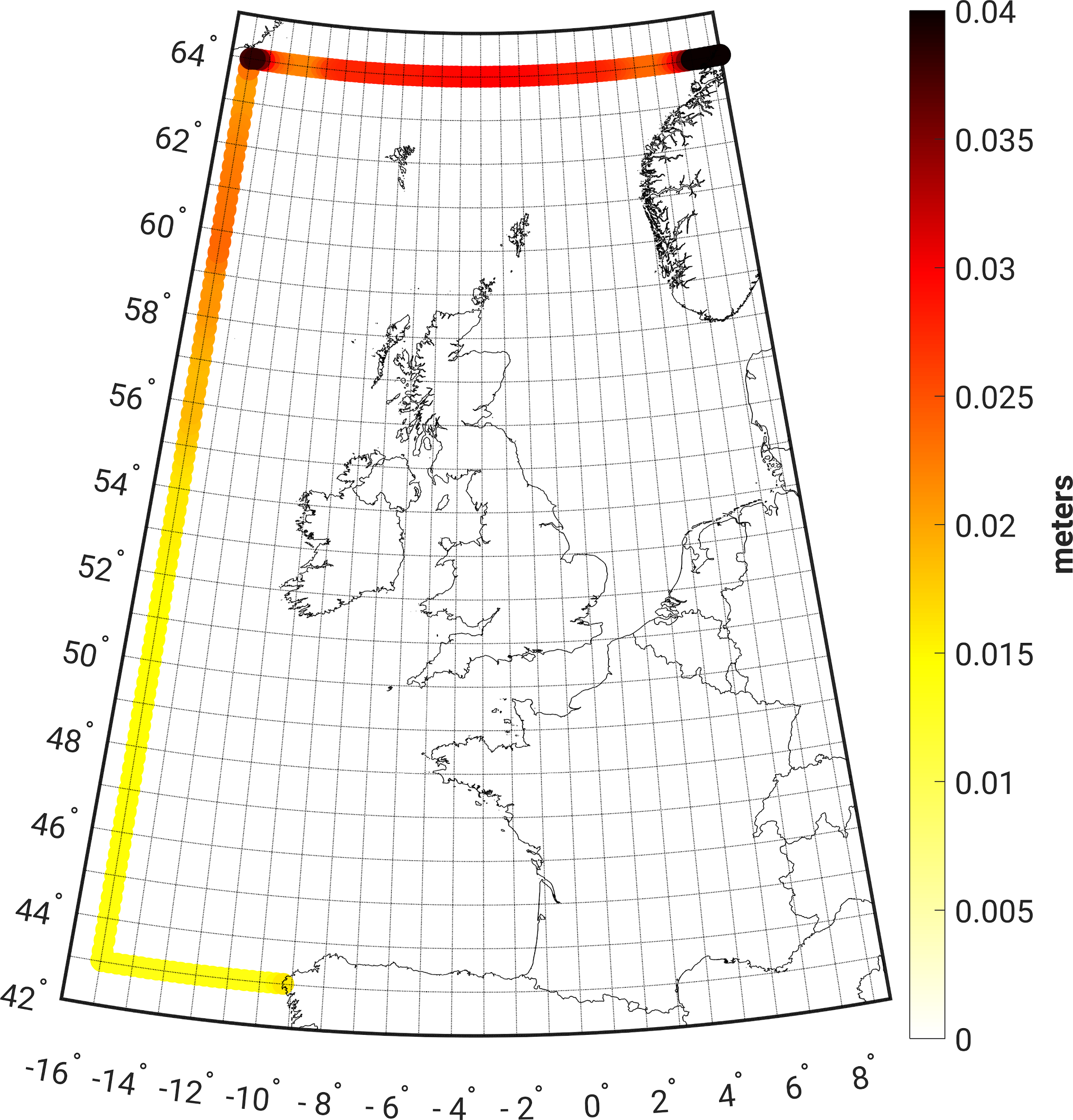
Fig. 2: Root-mean-square values of the differences between the IBC and DAC along the DCSMv6’s open boundaries over the period January 1993 - January 2015. The DAC are produced by the CLS Space Oceanography Division using the MOG2D model from Legos and distributed by Aviso, with support from CNES. The IBC are computed using data from the interim reanalysis project ERA-Interim (Dee et al. 2011).
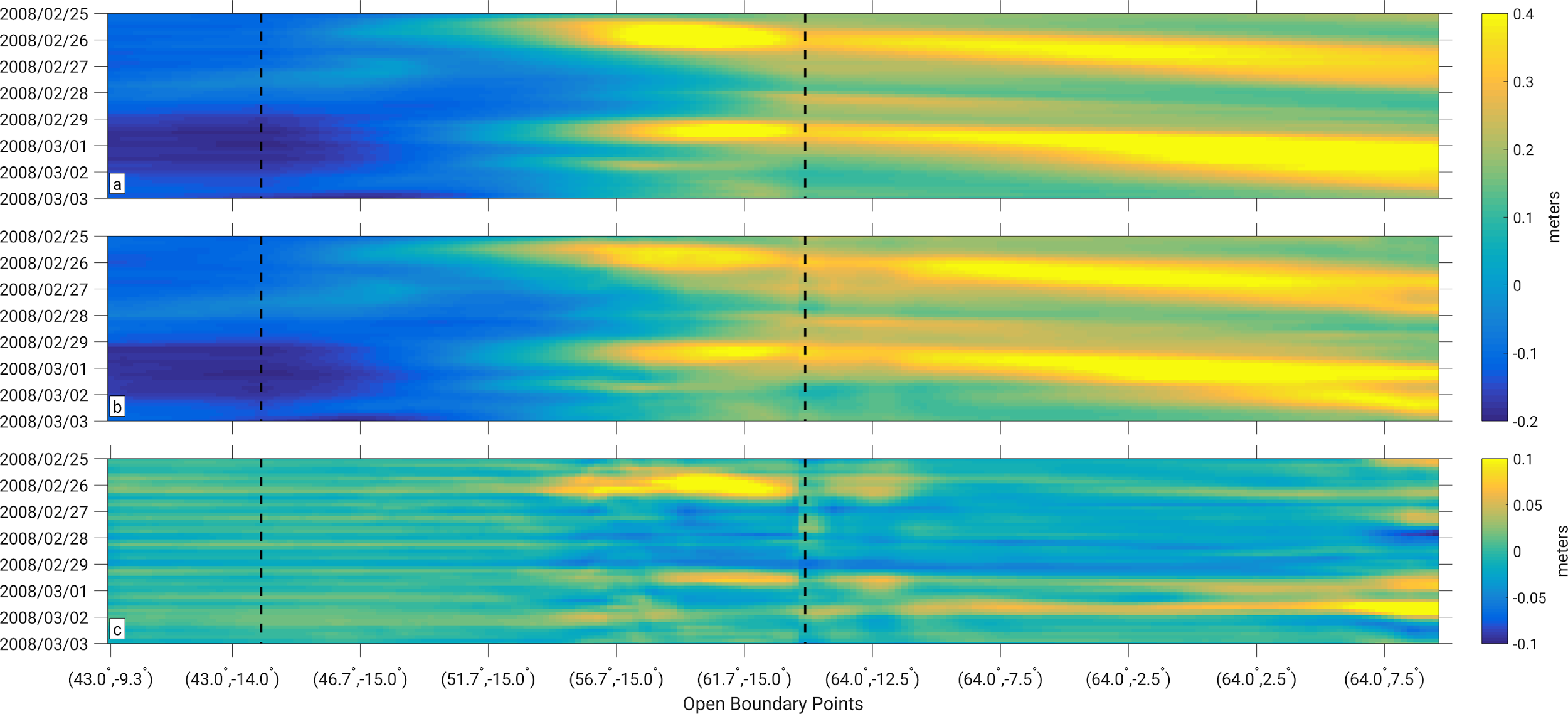
Fig. 3: Time series of the IBC (panel a) and DAC (panel b) along the open sea boundaries over the period February 25, 2008 - March 3, 2008. Panel c shows the time series of the differences between the IBC and DAC. The black dashed lines indicate the corners of the model domain.
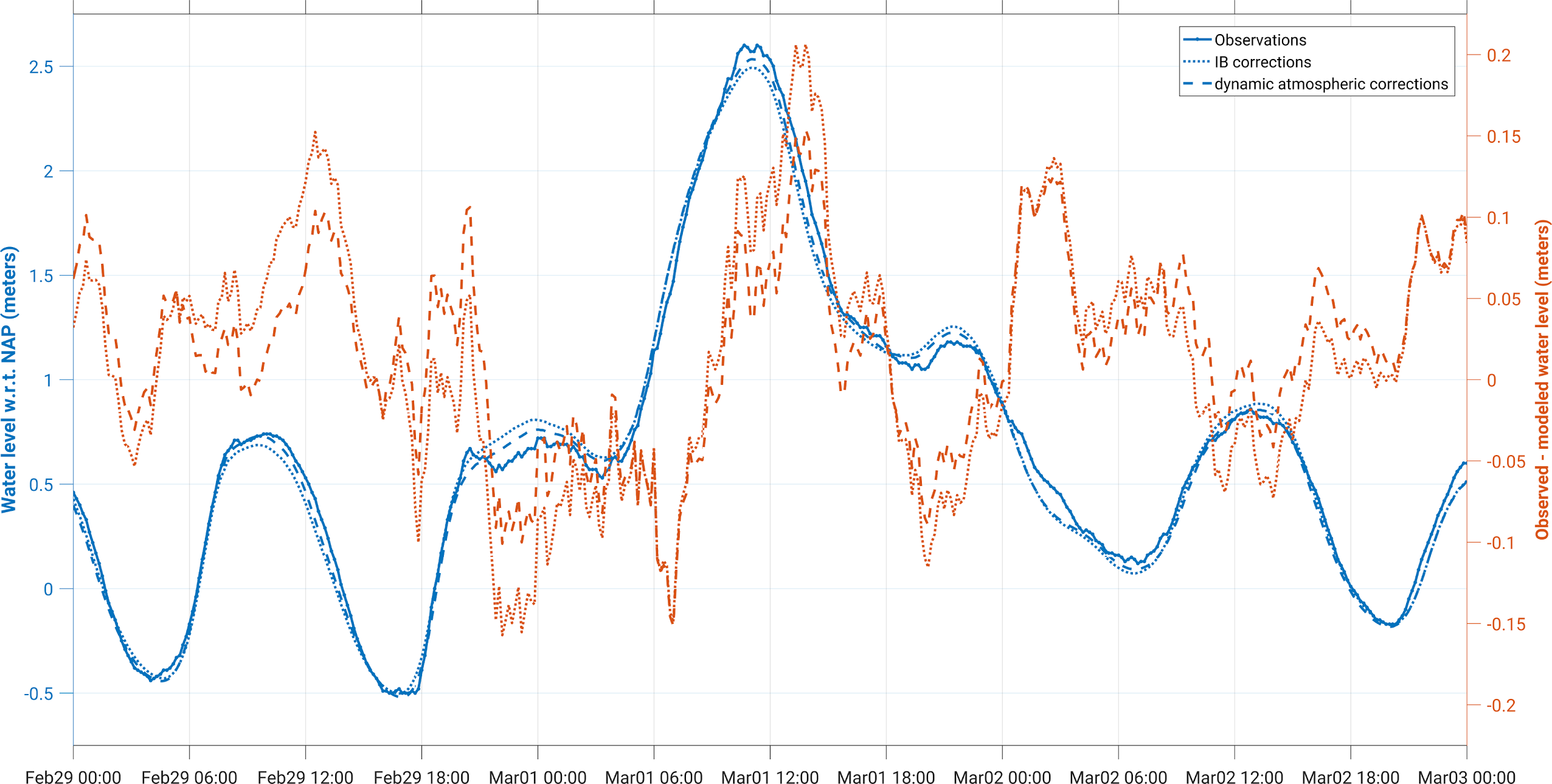
Fig. 4: The left y-axis shows the time series of observed and modeled water levels in Den Helder. The right y-axis shows their differences. The dotted and dashed lines refer to the setups where respectively the IBC and DAC are used as approximation of the surge water levels along the open sea boundaries.
FAST4Nl
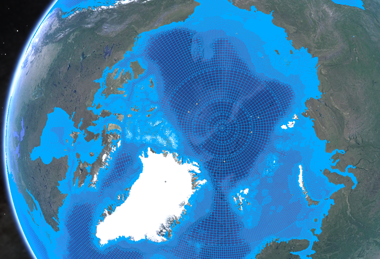
The Arctic TWL model to be developed in this project will be based on the in-house developed GTSM. Contrary to the extended HYCOM developed by Arbic et al. (2010, 2012), the GTSM uses an unstructured spherical grid, to represent coastal areas in more detail (~5 km resolution) than open oceans (50 km resolution). The model was calibrated and validated against about 300 coastal tide gauges and tides derived from satellite altimeter data. Recent developments include a new formulation for the self-attraction and loading term (Irazoqui Apecechea et al. 2017), an improved formulation for dissipation by internal tides and increased resolution especially over steep topography (De Kleermaeker et al. 2017). In this project, we will develop i) the physics needed to model the water level variations in ice-covered seas, ii) a method to account for the baroclinic water level variations, which are not yet included in the GTSM, and iii) a data assimilation technique and scheme to calibrate the model using novel synthetic aperture radar (SAR) altimeter data. The project consists of four work packages that are briefly described below.
WP 1: Develop Arctic component of GTSM
The first WP aims to develop the Arctic component of the GTSM. Based on a new bathymetric data set, we will refine the unstructured mesh where needed and update the model bathymetry. Furthermore, the missing contributions to the TWLs will be added as well as the physics needed to model the water level variations in ice-covered seas.
Contact: Prof. dr. ir. M. (Martin) Verlaan - info@fast4nl.nl
WP 2: Calibrate & validate model using SAR altimetry
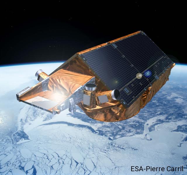
The main objectives of WP2 are to calibrate the model using data assimilation and to validate the model. Both the calibration and validation will be done using TWLs acquired at tide gauges and by the CryoSat-2 (Wingham et al., 2006) and Sentinel-3 (Donlon et al. 2012) satellites. Both satellites provide a good coverage of the Arctic waters and, most importantly, are equipped with a Synthetic Aperture Radar altimeter. The latter provides data with a much higher along-track resolution than a traditional pulse-limited radar, which is particularly useful to discriminate between sea ice floes and ocean leads. Moreover, CryoSat-2 data allows to obtain accurate measurements of the floating sea ice thickness that will be used to validate our input data sets.
Contact: Dr. ir. D.C. (Cornelis) Slobbe - info@fast4nl.nl
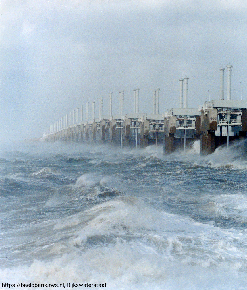
WP 3: Forecast Arctic tides and surges and assess their impact on water levels in the Netherlands
The main objective of WP3 is to improve storm surge forecasting in the Netherlands by improving the water levels along the open sea boundaries. In the current operational system, the prescribed water levels are obtained by summing the tidal and surge water levels (Zijl et al. 2013). The first are specified as tidal constituents, the latter are approximated using the inverted barometer correction (IBC). The specific research question we will address is under what conditions the IBC is not a good approximation of the Arctic surge? Further improvements of the open boundary conditions will be obtained by assimilating near real-time Sentinel-3 altimeter data. The latter are available in less than three hours and offer decimeter accuracy (European Space Agency 2012). Using these two model setups, we will quantify the impact of improved forecasts of Arctic tides and surges on storm surge forecasts in Dutch waters. In doing so, we will conduct both hindcasts and forecasts. The impact will be assessed by comparing model results to observations from a selection of Dutch tide gauges. We focus both on the surge amplitude and the timing of peak water level.
Contact: Dr. ir. D.C. (Cornelis) Slobbe - info@fast4nl.nl
.jpg)
WP 4: Project the impact of Arctic sea ice decline on tides and surges in the Arctic and the North Sea
In WP4 we will assess the impact of the (projected) Arctic sea ice decline on global tides and surges. Specifically, we will focus on the Arctic waters and the North Sea. The impact is quantified i) by linking modeled/observed changes in tide/surge over the last decades to the corresponding decline of the Arctic sea ice, and ii) by making projections of tides and surges based on projections of the Arctic sea ice decline.
Contact: Prof. dr. ir. M. (Martin) Verlaan - info@fast4nl.nl
References
- Arbic, B.K., A.J. Wallcraft, and E.J. Metzger. (2010). Concurrent simulation of the eddying general circulation and tides in a global ocean model. Ocean Modelling, 32:175–187, http://dx.doi.org/10.1016/j.ocemod.2010.01.007.
- Arbic, B.K., J.G. Richman, J.F. Shriver, P.G. Timko, E.J. Metzger, and A.J. Wallcraft. 2012. Global modeling of internal tides within an eddying ocean general circulation model. Oceanography 25(2):20–29, http://dx.doi.org/10.5670/oceanog.2012.38.
- ASSESSMENT, ARCTIC CLIMATE IMPACT (ACIA). (2005). Impacts of a warming Arctic: Arctic climate impact assessment, scientific report.
- Atkinson, D. E. (2005), Observed storminess patterns and trends in the circum-Arctic coastal regime, Geo Mar. Lett., 25, 98–109, doi:10.1007/s00367-004-0191-0.
- Barnhart, K. R., Overeem, I., & Anderson, R. S. (2014). The effect of changing sea ice on the physical vulnerability of Arctic coasts. The Cryosphere, 8(5), 1777-1799.
- Blauw, A. N., Beninca, E., Laane, R. W., Greenwood, N., & Huisman, J. (2012). Dancing with the tides: fluctuations of coastal phytoplankton orchestrated by different oscillatory modes of the tidal cycle. PloS one, 7(11), e49319.
- Carrère, L., and F. Lyard, 2003: Modeling the barotropic response of the global ocean to atmospheric wind and pressure forcing—Comparisons with observations. Geophys. Res. Lett., 30, 1275. doi:10.1029/2002GL016473.
- Chang, E. R., Veeneklaas, R. M., & Bakker, J. P. (2007). Seed dynamics linked to variability in movement of tidal water. Journal of Vegetation Science, 18(2), 253-262.
- Dee, D. P., Uppala, S. M., Simmons, A. J., Berrisford, P., Poli, P., Kobayashi, S., ... & Bechtold, P. (2011). The ERA‐Interim reanalysis: Configuration and performance of the data assimilation system. Quarterly Journal of the royal meteorological society, 137(656), 553-597.
- Dittmann, S. (Ed.). (1999). The Wadden Sea ecosystem. Berlin: Springer-Verlag.
- Donlon, C., Berruti, B., Buongiorno, A., Ferreira, M.H., Féménias, P., Frerick, J., Goryl, P., Klein, U., Laur, H., Mavrocordatos, C. and Nieke, J. (2012). The global monitoring for environment and security (GMES) sentinel-3 mission. Remote Sensing of Environment, 120, 37-57.
- Duran-Matute, M., Gerkema, T., De Boer, G. J., Nauw, J. J., & Gräwe, U. (2014). Residual circulation and freshwater transport in the Dutch Wadden Sea: a numerical modelling study. Ocean Science, 10(4), 611-632.
- European Space Agency. (2012). Sentinel-3: ESA’s Global Land and Ocean Mission for GMES Operational Services (ESA SP-1322/3, October 2012), ISBN 978-92-9221-420-3, Noordwijk: ESA Communications, available online https://sentinel.esa.int/documents/247904/351187/ S3_SP-1322_3.pdf.
- Farahani, H. H., Slobbe, D. C., Klees, R., & Seitz, K. (2016). Impact of accounting for coloured noise in radar altimetry data on a regional quasi-geoid model. Journal of Geodesy, 1-16. doi:10.1007/s00190-016-0941-6
- Frederikse, T., R. Riva, D. C. Slobbe, T. Broerse, and M. Verlaan (2016), Estimating decadal variability in sea level from tide gauge records: An application to the North Sea, J. Geophys. Res. Oceans, 121, 1529–1545, doi:10.1002/2015JC011174.
- Fretwell, P.; Pritchard, H. D; Vaughan, D. G; Bamber, J. L; Barrand, N. E; Bell, R.; et al.(2013). Bedmap2: improved ice bed, surface and thickness datasets for Antarctica. The Cryosphere, 7(1), 375 - 393. doi: 10.5194/tc-7-375-2013. UC Irvine: Retrieved from: http://escholarship.org/uc/item/1140z46m
- Gerritsen H, de Vries H, Philippart M (1995) The Dutch continental shelf model. In: Lynch DR, Mooers CNK (eds) Quantitative skill assessment for coastal ocean models. Coastal estuarine studies, vol 47. AGU, Washington, DC, pp 425–467.
- Godin, G. (1986). Modification by an ice cover of the tide in James Bay and Hudson Bay. Arctic, 65-67.
- Greatbatch, R. J. (1994). A note on the representation of steric sea level in models that conserve volume rather than mass. Journal of Geophysical Research: Oceans, 99(C6), 12767-12771.
- Hazeleger, W., Wang, X., Severijns, C., Ştefănescu, S., Bintanja, R., Sterl, A., Wyser, K., Semmler, T., Yang, S., Van den Hurk, B., Van Noije, T. (2012). EC-Earth V2. 2: description and validation of a new seamless earth system prediction model. Climate dynamics, 39(11), 2611-2629.
- Irazoqui Apecechea, M.I., Verlaan, M., Zijl, F., Le Coz, C., & Kernkamp, H. (2017). Effects of Self-Attraction and Loading in a regional scale: A test case for the Northwest European Shelf, accepted for publication Ocean Dynamics.
- Jakobsson, M., L. A. Mayer, B. Coakley, J. A. Dowdeswell, S. Forbes, B. Fridman, H. Hodnesdal, R. Noormets, R. Pedersen, M. Rebesco, H.-W. Schenke, Y. Zarayskaya A, D. Accettella, A. Armstrong, R. M. Anderson, P. Bienhoff, A. Camerlenghi, I. Church, M. Edwards, J. V. Gardner, J. K. Hall, B. Hell, O. B. Hestvik, Y. Kristoffersen, C. Marcussen, R. Mohammad, D. Mosher, S. V. Nghiem, M. T. Pedrosa, P. G. Travaglini, and P. Weatherall, The International Bathymetric Chart of the Arctic Ocean (IBCAO) Version 3.0, Geophysical Research Letters, doi: 10.1029/2012GL052219.
- Jeffreys, H. (1916). Causes contributory to the Annual Variation of Latitude.(Plate 8.). Monthly Notices of the Royal Astronomical Society, 76(6), 499-525.
- Kagan, B. A., & Sofina, E. V. (2010). Ice-induced seasonal variability of tidal constants in the Arctic Ocean. Continental Shelf Research, 30(6), 643-647.
- De Kleermaeker S., M. Verlaan, T. Mortlock, J. Lima Rego, M.I. Irazoqui Apecechea ,K. Yan and D. Twigt. Global-to-local scale modelling of storm surge risk in Southeast Australia. Submitted to Coasts and Ports 2017
- Kokelj, S. V., T. C. Lantz, S. Solomon, M. F. J. Pisaric, D. Keith, P. Morse, J. R. Thienpont, J. P. Smol, and D. Esagok (2012), Utilizing multiple sources of knowledge to investigate northern environmental change: Regional ecological impacts of a storm surge in the outer Mackenzie Delta, N.W.T., Arctic, 65, 257–272.
- Kowalik, Z., & Untersteiner, N. (1978). A study of the M2 tide in the Arctic Ocean. Deutsche Hydrografische Zeitschrift, 31(6), 216-229. doi:10.1007/BF02226539.
- Kowalik, Z. (1981). A Study of the M-2 Tide in the Ice-Covered Arctic Ocean. Modeling, Identification and Control, 2(4), 201-223.
- Kwok, R., and D. A. Rothrock (2009), Decline in Arctic sea ice thickness from submarine and ICESat records: 1958–2008, Geophys. Res. Lett., 36, L15501, doi:10.1029/2009GL039035.
- Lintern, D. G., Macdonald, R. W., Solomon, S. M., & Jakes, H. (2013). Beaufort Sea storm and resuspension modeling. Journal of Marine Systems, 127, 14-25.
- Lynch, D. R., and W. G. Gray, 1979: A wave equation model for finite element tidal computations. Comput. Fluids, 7, 207–228.
- Madec G (2008), NEMO ocean engine. Note du Pole de modélisation, Institut Pierre-Simon Laplace (IPSL), France, No 27 ISSN No 1288–1619
- Manson, G. K., and S. M. Solomon (2007), Past and future forcing of Beaufort Sea coastal change, Atmos.-Ocean, 25, 107–122.
- Mathers, E. L., & Woodworth, P. L. (2001). Departures from the local inverse barometer model observed in altimeter and tide gauge data and in a global barotropic numerical model. Journal of Geophysical Research: Oceans, 106(C4), 6957-6972.
- Meier, W. N. (2017). Losing Arctic sea ice: observations of the recent decline and the long‐term context. Sea Ice, 290-303.
- Mouthaan EEA, Heemink AW, Robaczewska KB (1994) Assimilation of ERS-1 altimeter data in a tidal model of the continental shelf. Deutsche Hydrographische Zeitschrift 36(4):285–319.
- Muis, S., Verlaan, M., Winsemius, H. C., Aerts, J. C., & Ward, P. J. (2016). A global reanalysis of storm surges and extreme sea levels. Nat. Commun. 7:11969 doi: 10.1038/ncomms11969.
- Murty, T. S. (1985). Modification of hydrographic characteristics, tides, and normial modes by ice cover. Marine Geodesy, 9(4), 451-468.
- Overeem, I., R. S. Anderson, C. W. Wobus, G. D. Clow, F. E. Urban, and N. Matell (2011), Sea ice loss enhances wave action at the Arctic coast, Geophys. Res. Lett., 38, doi:10.1029/2011GL048681.
- Padman, L., Fricker, H. A., Coleman, R., Howard, S., & Erofeeva, L. (2002). A new tide model for the Antarctic ice shelves and seas. Annals of Glaciology, 34(1), 247-254.
- Parke, M. E., R. H. Stewart, D. L. Farless, and D. E. Cartwright (1987), On the choice of orbits for an altimetric satellite to study ocean circulation and tides, J. Geophys. Res., 92(C11), 11693–11707, doi:10.1029/JC092iC11p11693.
- Perovich, D. K., & Richter-Menge, J. A. (2009). Loss of sea ice in the Arctic. Annual Review of Marine Science, 1, 417-441.
- Philippart ME, Gebraad AW, Scharroo R, Roest MRT, Vollebregt EAH, Jacobs A, van den Boogaard HFP, Peters HC (1998). DATUM2: data assimilation with altimetry techniques used in a tidal model, 2nd program. Tech. rep., Netherlands Remote Sensing Board.
- Pickering, M. D., Horsburgh, K. J., Blundell, J. R., Hirschi, J. M., Nicholls, R. J., Verlaan, M., & Wells, N. C. (2017). The impact of future sea-level rise on the global tides. Continental Shelf Research, doi: 10.1016/j.csr.2017.02.004.
- Ricker, R., Hendricks, S., Helm, V., & Gerdes, R. (2015). Classification of CryoSat-2 radar echoes. In Towards an Interdisciplinary Approach in Earth System Science (pp. 149-158). Springer International Publishing.
- Ricker, R., Hendricks, S., & Beckers, J. F. (2016). The Impact of Geophysical Corrections on Sea-Ice Freeboard Retrieved from Satellite Altimetry. Remote Sensing, 8(4), 317.
- Rothrock, D. A., Yu, Y., & Maykut, G. A. (1999). Thinning of the Arctic sea‐ice cover. Geophysical Research Letters, 26(23), 3469-3472.
- Scharroo, R., 2012. RADS version 3.1: User Manual and Format Specification. Delft University of Technology, http://rads.tudelft.nl/rads/radsmanual.pdf.
- Sepp, M., and J. Jaagus (2011), Changes in the activity and tracks of Arctic cyclones, Clim. Change, 105, 577–595.
- Slobbe, D. C., Verlaan, M., Klees, R., & Gerritsen, H. (2013a). Obtaining instantaneous water levels relative to a geoid with a 2D storm surge model. Continental Shelf Research, 52, 172-189.
- Slobbe, D. C., Klees, R., Verlaan, M., Dorst, L. L., & Gerritsen, H. (2013b). Lowest astronomical tide in the North Sea derived from a vertically referenced shallow water model, and an assessment of its suggested sense of safety. Marine Geodesy, 36(1), 31-71.
- Slobbe, D. C., Klees, R., & Gunter, B. C. (2014a). Realization of a consistent set of vertical reference surfaces in coastal areas. Journal of Geodesy, 88(6), 601-615.
- Slobbe, D.C., R. Klees (2014b). “The impact of the dynamic sea surface topography on the quasi-geoid in shallow coastal waters.” Journal of Geodesy 88(3): 241-261, DOI 10.1007/s00190-013-0679-3.
- Slobbe, D. C., Klees, R., Verlaan, M., Zijl, F., Farahani, H. H. (2016). Height system connection between island and mainland using a hydrodynamic model. Paper presented at the International Symposium on Gravity, Geoid and Height Systems 2016, Thessaloniki, Greece.
- St‐Laurent, P., Saucier, F. J., & Dumais, J. F. (2008). On the modification of tides in a seasonally ice‐covered sea. Journal of Geophysical Research: Oceans, 113(C11).
- Stammer, D., Ray, R. D., Andersen, O. B., Arbic, B. K., Bosch, W., Carrère, L., ... & Erofeeva, S. Y. (2014). Accuracy assessment of global barotropic ocean tide models. Reviews of Geophysics, 52(3), 243-282.
- Stormvloedwaarschuwingsdienst (2008). VERSLAG VAN DE STORMVLOED van 1 maart 2008 (SR89), available online at: http://projects.knmi.nl/maritiem/WAQUA/SVSD/ (In Dutch).
- Stroeve, J., M. M. Holland, W. Meier, T. Scambos, and M. Serreze (2007), Arctic sea ice decline: Faster than forecast, Geophys. Res. Lett., 34, L09501, doi:10.1029/2007GL029703.
- De Swart, H. E., & Zimmerman, J. T. F. (2009). Morphodynamics of tidal inlet systems. Annual review of fluid mechanics, 41, 203-229.
- Verboom GK, de Ronde JG, van Dijk RP (1992) A fine grid tidal flow and storm surge model of the North Sea. Cont Shelf Res 12:213–233.
- Verlaan, M., De Kleermaeker S., & Buckman L. (2015). GLOSSIS: Global Storm Surge Forecasting and Information System. Paper presented at Australasian Coasts & Ports Conference 2015, 15 - 18 September 2015, Auckland, New Zealand.
- Vermaire, J. C., M. F. J. Pisaric, J. R. Thienpont, C. J. Courtney Mustaphi, S. V. Kokelj, and J. P. Smol (2013), Arctic climate warming and sea ice declines lead to increased storm surge activity, Geophys. Res. Lett., 40, 1386–1390, doi:10.1002/grl.50191.
- Vousdoukas, M. I., Mentaschi, L., Voukouvalas, E., Verlaan, M. and Feyen, L. (2017), Extreme sea levels on the rise along Europe's coasts. Earth's Future. doi:10.1002/2016EF000505.
- Wingham, D. J., Francis, C. R., Baker, S., Bouzinac, C., Brockley, D., Cullen, R., ... & Phalippou, L. (2006). CryoSat: A mission to determine the fluctuations in Earth’s land and marine ice fields. Advances in Space Research, 37(4), 841-871.
- Wunsch, C., & Stammer, D. (1997). Atmospheric loading and the oceanic “inverted barometer” effect. Reviews of Geophysics, 35(1), 79-107.
- Zijl, F., Verlaan, M., & Gerritsen, H. (2013). Improved water-level forecasting for the Northwest European Shelf and North Sea through direct modelling of tide, surge and non-linear interaction. Ocean Dynamics, 63(7), 823-847.
- Zijl, F., Sumihar, J., & Verlaan, M. (2015). Application of data assimilation for improved operational water level forecasting on the northwest European shelf and North Sea. Ocean Dynamics, 65(12), 1699-1716.
- Zijl, F., Sumihar, J., & Verlaan, M. (2015b). Improved operational water - level forecasting on the Northwest European Shelf and North Sea (DCSMv6 and DCSMv6 - ZUNOv4). eSurge User Consultation Workshop, Delft, January 20, 2015. http://www.storm-surge.info/sites/storm-surge.info/files/Delft%2006%20-%20Zijl.pdf